A Not So Gentle Introduction to PPO & GRPO

If you’re reading this, I’m stuck on a 9-hour SFO-LHR flight with nothing else to do but munch on some high-calorie snacks and endure a mediocre movie selection. Since I have nothing better to do and have been putting it off for quite some time, I figured now’s as good a time as any to finally do a deep dive on the DeepSeek R1 paper.

The paper shows some impressive results using something called Group Relative Policy Optimization (GRPO), which is basically a simplified version of Proximal Policy Optimization (PPO). I’ve always found these reinforcement learning papers a bit dense, so I’m going to break this down step by step, starting from the basics.

My approach to tackling complex topics is building intuition rather than just memorizing formulas. So yes, we’ll be looking at lots of equations (medical school definitely didn’t prepare me for this), but I’ll attempt to walk through each concept, explain why it matters, and try to connect everything together in a way that actually makes sense.

Let’s get into it!

Pre-training vs Post-Training

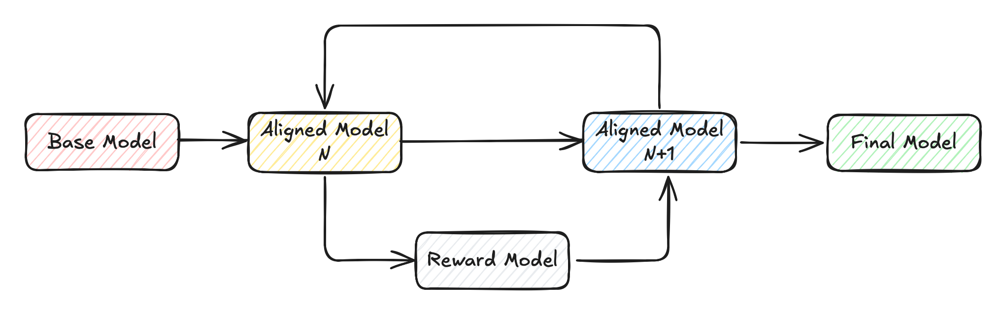Figure 1: A simplified overview of a modern post-training pipeline. Courtesy of the RLHF Book

The training of Large Language Models (LLMs) has traditionally been separated into two distinct phases:

• Pre-training: The initial phase where models learn language structure and knowledge from vast text corpora through self-supervised learning, primarily using next-token prediction. The model learns to predict what comes next in a sequence, developing statistical patterns of language and absorbing factual knowledge along the way. During this phase, models develop their fundamental capabilities for text prediction and generation, but lack specific alignment with human instructions or preferences.

• Post-training: A set of techniques to make language models more useful. These can be broadly categorized into:

  • Instruction/Supervised fine-tuning (IFT/SFT) which concerns itself with teaching models formatting and base instruction following.
  • Preference fine-tuning (PreFT) where models are aligned to human preferences that are hard to quantify, such as style.
  • Reinforcement Fine-tuning (RFT), where the performance of models in verifiable domains is improved.

The evolution from raw pre-trained models to useful assistants relies heavily on these post-training techniques, with RFT becoming increasingly central to competitive model development. Notably, one of the more surprising aspects of the DeepSeek paper, is that their R1 model applies RFT directly to the base model, skipping SFT/PreFT entirely.

Problem Formulation

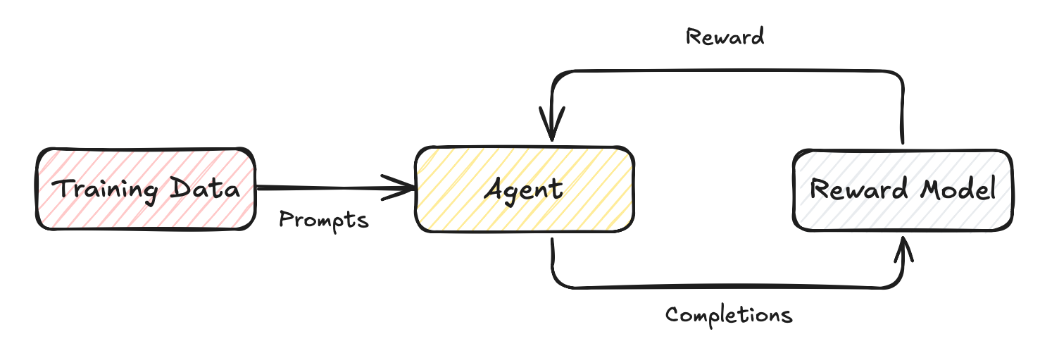Figure 2: The modified reinforcement learning setup for LLMs

In reinforcement learning, an agent takes actions, $a$, sampled from a policy $\pi$, with respect to the state of the environment $s$, to maximize reward $r$. A lot of these terms can seem a little alien so here are some quick definitions:

• Action ($a$): An action undertaken by an agent in an environment, where $a \in A$, the set of all possible actions in an environment.
• Policy ($\pi$): A policy is the strategy an agent follows to decide which action to take in a given state, or $\pi(a\mid s)$.
• State ($s$): The current state (read configuration) of the environment, where $s \in S$, where $S$ is a set of all possible states of the environment.
• Reward ($r$): A scalar value denoting the desirability or goodness of an action or state.
• Trajectory ($\tau$): A sequence of states and actions $(s_0, a_0, s_1, a_1, ...)$ that occurs when an agent interacts with an environment following a specific policy. Hence the goal of an RL agent is to solve the following:

$$J(\pi) = \mathbb{E}_{\tau \sim \pi} \left[ \sum_{t=0}^{\infty} \gamma^t r(s_t, a_t) \right]$$

which basically translates to saying: "Find the policy (strategy) that maximizes the expected sum of discounted rewards over time." The agent aims to identify a strategy $\pi$ that, when followed, yields the highest possible cumulative reward across all possible trajectories $\tau$ through the environment. The discount factor $\gamma$ (usually between 0 and 1) ensures that immediate rewards are valued more highly than distant ones, reflecting the intuition that a reward now is worth more than uncertain rewards later.

With a few modifications, we can turn this traditional RL problem formulation into one that more closely resembles the ones used in language modeling:

1. Since we aim to teach a model to amplify certain behaviors and eliminate others, it is common to use a learned model rather than an environment reward function. In other words, instead of having humans manually rate the outputs of our model, we have our annotators rate a small portion of the model’s outputs, then train a model to predict these annotators’ preferences. Et voilà, our reward model. Don’t fret, we’ll get to the implementation details of this model in a few sections.
2. Unlike traditional RL, there are no state transitions in language model training. The “state” is simply a prompt from our dataset, and the “action” is the model’s complete response to that prompt. The model generates a response, receives feedback, and then moves to a new, unrelated prompt—there’s no continuing sequence where actions affect future states. This simplifies our approach considerably.
3. Rewards are attributed at the response level, not for individual tokens. This creates what’s often called a “bandit problem,” where the model receives just one reward signal for an entire sequence of generated tokens. This infrequent feedback makes it challenging to determine which specific parts of a response contributed most to its overall quality rating. For instance, if a response receives a low score, the model doesn’t immediately know which tokens or sentences were problematic.​​​​​​​​​​​​​​​​ Given these changes, our problem formulation can be simplified by removing the discount factor, time horizon, and using a reward model $r_\theta$:

$$J(\pi) = \mathbb{E}_{\tau \sim \pi} \left[ r_\theta(s_t, a_t) \right]$$

Reward Modeling

As mentioned in the previous section, reward models used in the post-training phase of LLMs serve as a proxy for environment rewards. But how do we train this model? Here we introduce the Bradley-Terry model of preference:

$$P(i > j) = \frac{p_i}{p_i + p_j}$$

Which measures the probability that two events $i$ and $j$ drawn from the same distribution satisfy the relation $i > j$. Breaking this down:

• $P(i > j)$ is the probability that option $i$ is preferred over option $j$.
• $p_i$ and $p_j$ are the “strength scores” of each option
• The fraction shows that as $p_i$ gets larger compared to $p_j$, the probability $P(i > j)$ approaches 1
• If both options have equal strength $p_i = p_j$, the probability becomes exactly 0.5

This model works like a sports ranking system: if Team A usually beats Team B, Team A gets a higher strength score. These scores let us convert subjective judgments (“this response is better than that one”) into concrete numbers that our models can use, while naturally handling the expectation that if A is better than B, and B is better than C, then A should be better than C.​​​​​​​​​​​​​​​​

As with all neural networks, we need to formulate a loss function that guides the learning process. To apply the Bradley-Terry model to language models, we make two key adaptations:

1. First, we create a reward model $r_\theta$ that takes a prompt $x$ and a response pair to output a single scalar score. This model is typically derived from a pre-trained language model with a small linear head attached.
2. Second, we treat the options $i$ and $j$ from the original formula as different possible responses $y_w$ and $y_l$ to the same prompt $x$, as the ‘winning’ (read preferred) and ‘losing’ responses respectively. Since neural networks output unconstrained values rather than strictly positive “strength” parameters, we apply the exponential function to ensure positivity. Putting it all together we obtain:

$$P(y_w > y_l) = \frac{\exp(r(y_w))}{\exp(r(y_w)) + \exp(r(y_l))}$$

To transform this model into a loss we can minimize to train our reward model, we apply standard maximum likelihood estimation. For those who’ve long forgotten their high school math, here’s the step-by-step transformation:

• We factor out $\exp(r_\theta(y_w))$ from both numerator and denominator:

$$\begin{aligned} P(y_w > y_l) &= \frac{\exp(r_\theta(y_w))}{\exp(r_\theta(y_w)) (1 + \frac{\exp(r_\theta(y_l))}{\exp(r_\theta(y_w))})} \\ &= \frac{1}{1 + \frac{\exp(r_\theta(y_l))}{\exp(r_\theta(y_w))}} \end{aligned}$$

Next, using the exponential property that $\frac{e^a}{e^b} = e^{a-b}$, we simplify:

$$\begin{aligned} P(y_w > y_l) &= \frac{1}{1 + \exp(r_\theta(y_l) - r_\theta(y_w))} \\ &= \frac{1}{1 + \exp(-(r_\theta(y_w) - r_\theta(y_l)))} \end{aligned}$$

This is exactly the sigmoid function $\sigma$ applied to the difference in rewards:

$$P(y_w > y_l) = \sigma(r_\theta(y_w) - r_\theta(y_l))$$

Since we want to maximize this probability in our training, and optimization algorithms typically minimize functions, we take the negative logarithm to arrive at our final loss function:

$$\mathcal{L}(\theta) = -\log(\sigma(r_\theta(x, y_w) - r_\theta(x, y_l)))$$

This is equivalent to the binary cross-entropy loss commonly used in classification tasks, effectively framing our preference learning problem as classifying which of two responses a human would prefer.​​​ ​​​​​​​​​​​​​

Policy Gradient Algorithms

Overview

Now that we have the ability to guide our model’s behavior via the signal obtained from the reward model, we need an effective way of updating the parameters of our language model. While the literature is rich with different approaches, we’ll only be focusing on policy gradients and introduce PPO and GRPO. But first, some definitions:

• Return ($G_t$): The total sum of rewards an agent receives from time step $t$ onward, with future rewards typically discounted by the discount factor $\gamma$: $G_t = R_{t+1} + \gamma R_{t+2} + \gamma^2 R_{t+3} + ... = \sum_{k=0}^{\infty} \gamma^k R_{t+k+1}$
• Value Function ($V(s)$): A learned function that estimates the expected total future reward $G_t$ an agent can obtain starting from state $s$ when following policy $\pi$. It quantifies "how good" it is to be in a specific state. $V^\pi(s) = \mathbb{E}_\pi[G_t | S_t = s]$
• Q-Function ($Q(s,a)$): The state-action value learned function that estimates the expected return from taking action $a$ in state $s$ and then following policy $\pi$ afterward. It answers "how good is it to take this specific action in this state?" $Q^\pi(s,a) = \mathbb{E}_\pi[G_t | S_t = s, A_t = a]$
• Advantage Function ($A(s,a)$): Measures how much better taking action $a$ in state $s$ is compared to the average action according to the current policy. It's defined as the difference between the Q-function and the Value function: $A^\pi(s,a) = Q^\pi(s,a) - V^\pi(s)$

So what does a policy gradient algorithm actually do? In plain English, policy gradient algorithms try to figure out "how good" different situations ($s$) are, based on a particular strategy ($\pi$) for making decisions, and then they adjust that strategy to maximize rewards. Mathematically, this translates to the following optimization:

$$J(\theta) = \sum_s d_\pi(s)V_\pi(s)$$

Where $d_\pi(s)$ is the stationary distribution of states under policy $\pi$, or the long-run frequency of visiting each state when following the policy. In simpler terms, this translates to "how often do we end up in state $s$" multiplied by "how valuable is state $s$". The objective function $J(\theta)$ sums this product across all possible states, effectively saying "maximize the values of states we're likely to visit."

To actually update our parameters we do, where $\alpha$ is the learning rate:

$$\theta \leftarrow \theta + \alpha \nabla_\theta J(\theta)$$

While simple at first glance, calculating $\nabla_\theta J(\theta)$ is where the complexity lies. Various formulations exist, but they generally follow this pattern:

$$g = \mathbb{E}\left[\sum_{t=0}^{\infty} \Psi_t \nabla_\theta \log \pi_\theta(a_t|s_t)\right]$$

Let's decode this:

• $\nabla_\theta \log \pi_\theta(a_t|s_t)$ tells us how to adjust our parameters to make action $a_t$ more likely in state $s_t$
• $\Psi_t$ is a weighting factor determining how strongly we should move in that direction.

Different choices for $\Psi_t$ give us different algorithms with different properties. Some of the more common choices for $\Psi_t$ include using the total reward of the trajectory ($\sum_{t=0}^{\infty} r_t$), the return ($G_t$), or the advantage function ($A^\pi(s_t, a_t)$) which is more commonly used.

And that’s it for vanilla policy gradient methods!

The Bias-Variance Tradeoff in Advantage Estimation

One of the trickiest parts of policy gradient methods is accurately estimating the advantage function. Remember, the advantage function $A^\pi(s_t, a_t)$ tells us how much better an action is compared to what we'd expect on average. It's like the "surprise" factor of a reward - if we got more reward than expected, the advantage is positive, and we want to make that action more likely in similar situations.

But how do we calculate this advantage in practice? Temporal Difference (TD) learning is simply a fancy name for learning from the difference between consecutive predictions - instead of waiting until the end of an episode to know if a decision was good, we make estimates based on what we observe along the way.

Let's look at a few ways we can estimate the advantage, each with its own tradeoff:

1. One-step Temporal Difference (TD) estimate: $\hat{A}_t^{(1)} = r_t + \gamma V(s_{t+1}) - V(s_t)$ where:

   • $r_t$ is the immediate reward at time step $t$
   • $\gamma$ is the discount factor that determines how much we value future rewards
   • $V(s_t)$ is the estimated value of the current state
   • $V(s_{t+1})$ is the estimated value of the next state

   This estimate has low variance but high bias - it only looks one step ahead, missing longer-term consequences. It basically says, "Was the immediate reward plus the value of the next state better than what I expected for this state?" It's quick and stable but shortsighted.

2. Monte Carlo (MC) estimate: $\hat{A}_t^{MC} = \sum_{i=t}^{T} \gamma^{i-t} r_i - V(s_t)$ where:

   • $\sum_{i=t}^{T} \gamma^{i-t} r_i$ is the sum of all future rewards, discounted by how far in the future they occur
   • $T$ is the final time step in the episode
   • $\gamma^{i-t}$ decreases the weight of rewards that are further in the future
   • $V(s_t)$ is again the estimated value of the current state

   This approach uses the full return from the trajectory, essentially saying, "Let's wait and see how all the rewards actually add up, then compare that to what we expected." It's unbiased (uses real returns) but has high variance (lots of randomness in long sequences) and is expensive to compute, especially for an LLM.

This is where Generalized Advantage Estimation (GAE) comes into play, with built-in bias-variance tradeoff. GAE works by combining multi-step prediction and weighted running average.

$$\hat{A}_t^{GAE(\gamma, \lambda)} = \sum_{l=0}^{\infty} (\gamma \lambda)^l \delta_{t+l}^V$$

where:

• $\delta_t^V = r_t + \gamma V(s_{t+1}) - V(s_t)$ is the TD error at time step $t$
• $\lambda \in [0,1]$ is the GAE parameter that controls the bias-variance tradeoff
• $\gamma$ is the same discount factor used in the previous formulas
• $\sum_{l=0}^{\infty}$ indicates we're summing over all future time steps

In short, GAE combines the best of both worlds by creating a weighted average of all possible n-step return estimates.

• When $\lambda = 0$: GAE equals the one-step TD estimate (high bias, low variance)
• When $\lambda = 1$: GAE equals the Monte Carlo estimate (low bias, high variance) In language models, GAE helps solve the credit assignment problem by providing a more stable advantage estimate that can attribute rewards to specific tokens even when feedback is sparse.

Proximal Policy Optimization (PPO)

With all of this background information out of the way, we’re finally ready to talk about PPO, which provides several stability improvements over vanilla policy optimization. While there are several variants of this algorithm out there, we’ll focus on the standard formulation:

$$J(\theta) = \min \left( \frac{\pi_\theta(a|s)}{\pi_{\theta_{old}}(a|s)}A, \text{clip}\left( \frac{\pi_\theta(a|s)}{\pi_{\theta_{old}}(a|s)}, 1 - \varepsilon, 1 + \varepsilon \right) A \right)$$

and per-token versions adapted specifically for language modeling:

$$J(\theta) = \frac{1}{|a|} \sum_{t=0}^{|a|} \min \left( \frac{\pi_\theta(a_t|s_t)}{\pi_{\theta_{old}}(a_t|s_t)}A_t, \text{clip}\left( \frac{\pi_\theta(a_t|s_t)}{\pi_{\theta_{old}}(a_t|s_t)}, 1 - \varepsilon, 1 + \varepsilon \right) A_t \right)$$

In the context of LLMs, $\pi_\theta$ represents the language model itself — specifically, the model's policy for generating text, parameterized by $\theta$. In practice, $\pi_\theta$ is the categorical distribution head at the final layer of the neural network. This distribution outputs probability values across the model's entire vocabulary (typically 50K-100K tokens), telling us how likely each potential next token is given the current context. When we talk about $\pi_\theta(a_t|s_t)$, we're referring to the probability (or log-probability for numerical stability) that the model assigns to generating token $a_t$ given the context $s_t$. For example, if the prompt is "The capital of France is" ($s_t$), the model's distribution head might assign a 0.92 probability to "Paris" ($a_t$), 0.03 to "Lyon," and spread the remaining probability mass across other tokens. During training, we can extract these token probabilities or log-probabilities directly from this distribution to compute our policy ratios. Now back to the equations!

At first glance, PPO is pretty complex and it may be difficult to parse at first glance, but let’s decompose it into its primary constituents:

1. The Policy Ratio $\frac{\pi_\theta(a|s)}{\pi_{\theta_{old}}(a|s)}$: The ratio between the probability of taking an action (read: generating a token) under the current policy and the probability under the old policy. Initially starts at $1$ for a new batch. If $ratio > 1$, the current policy favors a token more than the old policy, and if $ratio < 1$, the current policy favors a response less than the old policy. But why do we need this ratio? Let’s break it down:

   • Given an existing policy, we generate a large batch of rollout data.
   • We then sample a mini-batch of data from this data to update our model.
   • However after a few updates, our new policy may be very different from the old policy that generated the data, therefore becoming off-policy. To mitigate this, PPO introduces the policy ratio as an importance sampling correction term to reweight the advantage estimate and account for this shift in policy.

2. The Advantage Function $A$: We’ve covered this extensively already, but as a reminder, the advantage function estimates how much better an action is compared to the average action according to the current policy. Positive advantage indicates actions that performed better than expected, while negative advantage indicates worse-than-expected performance.

3. The Clipping Function $\text{clip}(\frac{\pi_\theta(a|s)}{\pi_{\theta_{old}}(a|s)}, 1 - \varepsilon, 1 + \varepsilon)$: This constrains the policy ratio to remain within the interval $[1-\varepsilon, 1+\varepsilon]$. The hyper-parameter $\varepsilon$ (typically 0.1 or 0.2) controls how much the policy can change in a single update step to prevent overconfidence. A few examples of how this works in practice with $\varepsilon = 0.2$:

   • If a new policy has a probability of $0.7$ for a token and the old policy has a probability of $0.5$ for that same token, the policy ratio is $1.4$, favoring the token. With clipping, the ratio is capped at $1.2$.
   • Similarly, if the new policy has a probability of $0.3$ for a token and the old policy has a probability of $0.5$, the policy ratio becomes $0.6$, disfavoring the token. With clipping, the ratio caps at $0.8$.

As you can see, this clipping mechanism prevents large updates to the policy, which can lead to instability and divergence in training. It effectively limits how much we can change our policy in one step, ensuring that we don't overcommit to an action.

4. The Min Operation: The objective takes the minimum of the unclipped and clipped objectives, creating an upper bound that prevents excessively large policy updates.

Together, these operations address one of the primary challenges in policy gradient methods: preventing destructively large updates (read: overconfidence) that could collapse performance. In the per-token adaptation, we introduce $\frac{1}{|a|}$ to average the value by the number of tokens in the response, and operate on log-probabilities for numeric stability. That’s it!

Group Relative Proximal Policy Optimization (GRPO)

GRPO, at the core of the DeepSeek paper, can be viewed as a derivative of the PPO algorithm with some optimizations, namely avoiding the need to learn a value function. Instead, GRPO assigns the same value to every token by estimating the group advantage, after sampling multiple completions for the same prompt. Intuitively, what we’re doing is comparing multiple answers to the same question within a batch, and teaching the model to become more like the answers marked as correct. We don’t need to train (and update) a separate value network calculating per-token rewards.

As before, let’s take a look at the objectives first, and then decompose them into manageable chunks to get a better appreciation of the changes. Since the loss is accumulated over a group of responses $\{a_1, a_2, …, a_G\}$ we get:

$$J(\theta) = \frac{1}{G} \sum_{i=1}^{G} \left( \min \left( \frac{\pi_\theta(a_i|s)}{\pi_{\theta_{old}}(a_i|s)} A_i, \text{clip} \left( \frac{\pi_\theta(a_i|s)}{\pi_{\theta_{old}}(a_i|s)}, 1 - \varepsilon, 1 + \varepsilon \right) A_i \right) - \beta D_{KL} (\pi_\theta || \pi_{ref}) \right)$$

with the expanded per-token loss computation:

$$J(\theta) = \frac{1}{G} \sum_{i=1}^{G} \frac{1}{|a_i|} \sum_{t=1}^{|a_i|} \left( \min \left( \frac{\pi_\theta(a_{i,t}|s_{i,t})}{\pi_{\theta_{old}}(a_{i,t}|s_{i,t})} A_{i,t}, \text{clip} \left( \frac{\pi_\theta(a_{i,t}|s_{i,t})}{\pi_{\theta_{old}}(a_{i,t}|s_{i,t})}, 1 - \varepsilon, 1 + \varepsilon \right) A_{i,t} \right) - \beta D_{KL} (\pi_\theta(\cdot|s_{i,t})|| \pi_{ref}(\cdot|s_{i,t})) \right)$$

with the advantage computation being:

$$A_i = \frac{r_i - \text{mean}(r_1, r_2, \cdots, r_G)}{\text{std}(r_1, r_2, \cdots, r_G)}$$

The equation should look very familiar at this point. Keeping in mind that for GRPO we are sampling multiple completions ($a_i$) and collecting multiple rewards $r_i$ from the same prompt $s$:

1. Group-Level Averaging $\frac{1}{G} \sum_{i=1}^{G}$: This term averages the loss across all $G$ responses sampled from the same prompt, creating a more stable training signal and reducing variance.
2. Min and Clipping Functions $\min \left( \frac{\pi_\theta(a_i|s)}{\pi_{\theta_{old}}(a_i|s)} A_i, \text{clip} \left( \frac{\pi_\theta(a_i|s)}{\pi_{\theta_{old}}(a_i|s)}, 1 - \varepsilon, 1 + \varepsilon \right) A_i \right)$: Similar to the core PPO mechanism, this function restricts large updates to the policy thereby penalizing overconfidence.
3. Kullback-Leibler (KL) divergence $\beta D_{KL} (\pi_\theta || \pi_{ref})$: The KL-divergence is the measure of the relative difference between two probability distributions. In this case, we’re penalizing the model from diverging too far from the original model policy (instead of just the model policy right before the current policy update in the min-clipping function) to prevent the model from forgetting knowledge or abilities acquired in other training/post-training steps. We need our helpful LLM to continue being a helpful LLM!

It’s important to note that KL-divergence penalty is not exclusive to GRPO but is also used in many other losses (e.g. PPO). I only mention it here as it is included as part of the GRPO loss function.

4. Group-Normalized Advantage Estimation $A_i = \frac{r_i - \text{mean}(r_1, r_2, \cdots, r_G)}{\text{std}(r_1, r_2, \cdots, r_G)}$: Arguably the most important aspect of GRPO, the group-normalized advantage calculates the normalized reward of each response within its group of responses.

And there we have it, a rather elegant solution to the credit assignment problem in RL, with 3 hours left to spare on my flight. Although GRPO is far from being a silver-bullet (e.g. if all of the answers within a group are homogenous), from an implementation perspective, it significantly reduces computational overhead compared to traditional PPO, since we’re no longer loading a value network (usually another LLM) in memory. If you found this breakdown helpful, I’d love to hear your thoughts. As for me, I’ll be spending the rest of this flight contemplating whether the airline pretzels are worth the salt intake.​​​​​​​​​​​​​​​​

Acknowledgements

A big thank you to Kyle Birnbaum, Kashif Rasul, and Quentin Gallouedec for their help in reviewing this post. I’m also grateful to Nathan Lambert, author of the RLHF Book, for their excellent work in making this complex topic more accessible.

Additional Resources

For additional reading, there are a lot of fantastic resources on this topic already out there. Here are a few of my recommendations:

• The RLHF Book
• A vision researcher’s guide to some RL stuff: PPO & GRPO
• Proximal Policy Optimization
• Advanced understanding of Group Relative Policy Optimization (GRPO)